The Hidden Cost of AI: A Deep Dive into Inference Optimization and Vector Databases

This is an advanced infrastructure guide for engineering teams and technical decision-makers. For beginner-friendly AI tool breakdowns, explore our other AI Unboxed articles.

Most conversations about AI cost focus on the wrong number. The price per million tokens on OpenAI’s pricing page is the visible cost; the one that gets pasted into spreadsheets, used in budget proposals, and cited in board presentations. The real cost of running AI at scale is what happens after the model is deployed: the per-request compute overhead, the GPU hours, the vector database storage and query bills, and the embedding regeneration cycles that nobody budgeted for because they didn’t know they existed. I’ve watched teams build AI products with detailed API cost models that were accurate to within 10% during development and wrong by 400% at production scale, not because their math was bad, but because inference optimization and retrieval infrastructure weren’t in the model at all. The result is a product that can’t survive its own growth.

This article unpacks the two categories of hidden AI cost that every engineering team eventually hits: inference optimization, the mechanics of how efficiently you run models, and vector databases, the retrieval infrastructure that RAG systems depend on. Each has a visible cost and a much larger hidden one. Consequently, whether you’re a startup shipping your first AI feature, a growth-stage company watching your GPU bill compound monthly, or an enterprise team evaluating AI infrastructure strategy, the frameworks and verified numbers in this guide give you what vendor pricing pages won’t: the complete picture, with the uncomfortable parts included.

The True Economics of AI Inference: What You’re Actually Paying For

Here’s the first thing most teams get wrong about AI inference cost: they treat the per-token API price as the full cost. It isn’t. The per-token price is the cost of outsourcing your inference to a provider that has already absorbed the burden of infrastructure, optimization, and operations.

When you move to self-hosted inference, the cost structure becomes more visible. At a practical level, it usually comes down to four components, and understanding each one helps you decide which optimization actually matters for your workload.

• Compute is the numerical work done during the model’s forward pass. It scales with model size and sequence length, and it is the part most teams think about first. Optimizations like quantization and distillation reduce the amount of compute required per token.

• Memory capacity is the GPU VRAM needed to hold model weights, the KV cache, and other runtime tensors. This is where model size becomes a hard constraint. A 70B model in FP16 requires roughly 140 GB just for weights, before accounting for cache and serving overhead. Quantization reduces that footprint and can make larger models feasible on fewer GPUs, depending on batch size and context length.

• Memory bandwidth is often the bottleneck that surprises people who have not profiled inference workloads. Generating each new token requires moving large amounts of data through GPU memory, and for bigger models, this can limit throughput as much as compute itself. Speculative decoding and continuous batching both help here by improving effective token throughput and reducing wasted GPU cycles.

• Idle time is GPU time spent waiting between requests. A GPU that sits idle still costs money, so utilization matters. Continuous batching exists largely to reduce this waste by keeping the GPU busy across more of the request lifecycle.

The Scale Reality Check

The Stanford HAI 2025 AI Index Report says inference costs for a GPT-3.5-level system fell by more than 280-fold between November 2022 and October 2024. The report is also widely cited for showing substantial annual improvements in hardware cost and energy efficiency. 

That sounds like the problem is solving itself. It isn’t, because usage has scaled faster than efficiency. 

A 280× improvement in per-token cost, combined with a 500× increase in token consumption, results in a higher total bill, not a lower one. At the company level, you’re competing on cost structure, not on the industry average.

At the startup scale, the cost is manageable but wasteful. At the growth scale, optimization is the difference between a sustainable product and one that burns cash. At the enterprise scale, a 75% cost reduction saves $4.3 million per year. The optimization techniques in the next section aren’t academic exercises. They’re the decisions that determine whether your product’s unit economics work.

One more thing worth saying plainly before we get into techniques: the most common naive optimization is switching from a 70B model to a 7B model. This reduces costs by 90% but also dramatically reduces quality for complex tasks. 

Production teams that make this switch without measuring quality impact find that customer satisfaction drops, error rates increase, and they spend engineering time on workarounds that erode the cost savings. Model downgrading without quality measurement isn’t optimization. It’s cost shifting.

Inference Optimization Techniques: The Technical Playbook

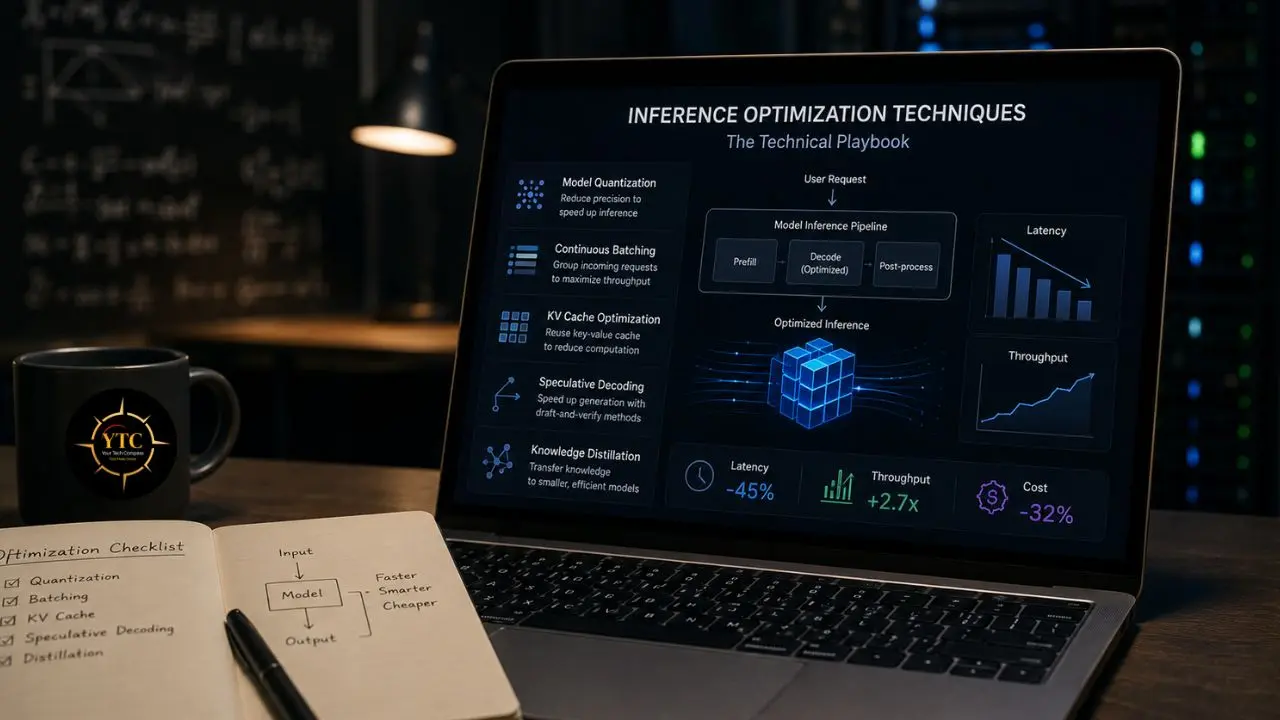
The five techniques below consistently deliver measurable ROI in production. I’ve organized them from fastest and lowest-effort to most involved because the right question isn’t “which technique is best”; it’s “which one moves the needle most for my team right now.” Work through them in order, measure quality at each step, and stop when the economics are right for your current scale.

Technique 1: Model Quantization (The Fastest Win)

Quantization converts model weights from high-precision floating-point formats (e.g., FP16 or FP32) to lower-precision formats such as INT8, FP8, or INT4. The mechanism is straightforward: instead of representing each weight as a 16-bit or 32-bit number, you represent it as an 8-bit or 4-bit number, using significantly less memory and enabling faster computation on hardware with lower-precision tensor cores.

On 7B–70B models, teams report 1.5–3× faster LLM inference simply by moving to mixed-precision quantization and optimized kernels. More importantly, the memory reduction changes what hardware you need. At FP16, a 70B model needs two A100s just for weights. At INT4, it fits on a single H100 with room for the KV cache and concurrent requests.

The current production standard in 2026: FP8 inference is now production-standard on H100/H200, with INT4 (AWQ, GPTQ, GGUF) enabling 70B models on consumer GPUs. FP4 on B200 via TensorRT-LLM adds a further 1.5–2× gain over FP8. More quantization error than FP8, so test against your eval suite before moving to production.

The Honest Trade-Off 

Quantized models can deviate more on long-context evaluation benchmarks. The accuracy hit matters more at INT4 than FP8. INT4 (GPTQ/AWQ) is suitable for lower-quality-sensitive workloads such as classification and summarization. Not recommended for complex reasoning tasks.

The Practical Rule 

Apply FP8 to H100/H200 hardware first; it’s essentially a free improvement. Evaluate INT4 specifically for your workload with your quality metrics. Never deploy quantized models without running your eval suite first.

Technique 2: Continuous Batching (Eliminating GPU Idle Time)

Traditional batching submits a batch of requests together, processes them all, and returns results when the slowest request finishes. The problem is autoregressive generation: different requests produce different numbers of tokens and finish at different times. Without continuous batching, GPU slots sit idle waiting for the last request in the batch to complete before the next batch can start.

Continuous batching (also called iteration-level scheduling) inserts new requests into open slots as soon as a previous request finishes. The GPU stays utilized throughout. vLLM and TensorRT-LLM achieving 5× inference efficiency through continuous batching is not a benchmark result from ideal conditions. It’s what teams consistently report when moving from naive batching to continuous batching in production systems.

Adjusting batch size dynamically based on incoming traffic reduces latency spikes during high-volume periods. The implementation decision is straightforward: vLLM handles continuous batching natively, and most managed inference providers (Fireworks AI, Together AI, Groq) have it built in. If you’re self-hosting without it, enabling it should be your first change.

Technique 3: KV Cache Optimization

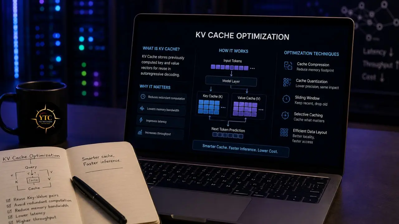
During autoregressive text generation, the model computes attention over all previously generated tokens for each new token. The KV (key-value) cache stores these attention computations so they don’t need to be recalculated. As context length grows, the KV cache grows proportionally, and managing it efficiently is one of the primary throughput bottlenecks in production inference.

vLLM’s PagedAttention manages KV cache the way a Linux kernel manages virtual memory: allocating cache pages on demand rather than reserving a fixed contiguous block per request from the start. This eliminates the memory waste from over-provisioning and allows more concurrent requests per GPU without running out of KV cache space. In practice, PagedAttention enables 2–4× more concurrent requests on the same hardware compared to naive KV cache management.

The context-length pricing implication connects directly here. Longer contexts mean larger KV caches, higher memory pressure, and either more GPU hours or shorter effective context lengths. Understanding how your application uses context length and whether you can reduce it through chunking, summarization, or retrieval design is as important as the KV cache implementation itself.

Technique 4: Speculative Decoding

Autoregressive generation is inherently sequential: each token depends on all previous tokens, so the model generates one token at a time. Speculative decoding breaks this serial dependency by using a small, fast “draft” model to generate candidate tokens, which a larger “target” model then verifies in parallel.

The key insight is that verification (checking whether the draft tokens are acceptable) is cheaper than generation, because the target model can evaluate multiple candidates simultaneously in a single forward pass rather than generating each token individually. Speculative decoding delivers 2–3× throughput for autoregressive generation.

The technique works best when the draft model’s output distribution closely matches the target model’s, which is most reliable for structured generation tasks like code, translation, and templated text. For a highly creative or unpredictable generation, the draft model acceptance rate drops and the throughput gains shrink. Evaluate it specifically for your generation tasks rather than assuming it is universally applicable.

Technique 5: Knowledge Distillation (The Highest-Impact, Highest-Effort Option)

Distillation trains a smaller “student” model to mimic the outputs of a larger “teacher” model. The goal is to compress knowledge into a form that requires significantly less compute to run while preserving enough quality for the specific task.

A growing body of work from 2024–2025 shows that well-distilled 7B–20B LLMs can handle many common chat and reasoning tasks that previously required much larger models, although the exact share depends on the workload and benchmark. Inference economics also favor smaller models, since a 14B deployment can often be run on fewer GPUs at materially lower hourly cost than a 70B deployment. 

The cost math is compelling. For instance: 70B on 8× H100 at $19.20/hr versus 14B on 2× H100 at $4.80/hr for comparable throughput on the target task. That’s a 4× cost reduction if your workload fits a distilled model.

The Honest Constraint 

Distillation is the highest-impact model change, but also the most work. It requires a clearly defined task scope, a rigorous quality evaluation framework, training infrastructure, and validation cycles. 

It’s not appropriate for every team or every timeline. The practical starting point for most teams is task-specific, fine-tuned smaller models, not full Zettelkasten-level distillation, but using open-source smaller models (Llama, Qwen, GLM families), fine-tuned on domain-specific data for your highest-volume task types.

For teams evaluating specific models for inference efficiency, our Qwen 3 review and GLM-4 review cover two of the most inference-efficient open-source model families available for self-hosting in 2026.

The Combined Impact

A single LLM inference request can become materially cheaper after optimization, though the exact price depends on model size, serving stack, and hardware. A 2025 ACL study found that proper LLM inference optimizations can reduce energy use by up to 73% compared with naive serving, thereby contributing to substantial cloud cost savings. 

The optimization sequence that delivers the best ROI in the shortest time: quantization first (lowest effort, highest immediate impact on memory and speed), then continuous batching (eliminates idle GPU waste), then KV cache optimization (unlocks more concurrent requests), then speculative decoding for high-volume generation workloads, then distillation for your highest-value task types where the quality bar is clearly defined.

The Inference Serving Decision: Build vs Buy vs Managed API

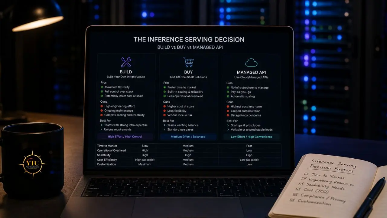
Once you understand the optimization techniques, the natural next question is where to apply them: on your own infrastructure or through a provider who’s already applied them. This is the decision that most significantly affects your actual monthly bill at scale.

📊 Inference Serving Options: Economics at a Glance

The Break-Even Analysis

Self-hosted inference on H100s can become economically attractive once managed API spend reaches a sufficiently high level, but the break-even point depends on GPU rental rates, utilization, staffing overhead, and the effort required to match the reliability of managed APIs. Below that point, the engineering cost of operating your own stack can outweigh the savings. 

A common production pattern is hybrid routing: use managed APIs for variable or frontier-model tasks and self-host smaller models for predictable, high-volume requests. For example, a product that routes 70% of simple queries to a self-hosted distilled model while forwarding 30% of complex queries to a managed frontier model can achieve a better cost-quality balance than either approach alone. 

For teams building on AWS infrastructure, our AWS AI tools and services guide covers the managed inference options within the AWS ecosystem, including SageMaker endpoints and Bedrock’s inference optimization features.

Vector Databases: The Hidden Infrastructure Cost in Every RAG System

Here’s a cost item that many AI teams underestimate until it shows up on a monthly bill: vector database infrastructure. The conversations I see most often go something like this: a team builds a RAG system during development, uses a free Chroma instance locally, deploys to production, and, six months later, is looking at a vector database bill that has become a meaningful share of their total AI infrastructure costs. 

Not because they were careless. Because the cost structure of vector databases at production scale differs sharply from what teams see during development.

Three things drive this gap. First, the embedding explosion: a single OpenAI text-embedding-3-large call produces a 3,072-dimensional vector. 

Store one million documents at this dimensionality, and you are already dealing with substantial raw vector storage before indexing overhead is counted. Production RAG systems routinely store far more vector data than teams initially expect once replicas, metadata, and index structures are included.

Second, the managed-versus-self-hosted cost gap widens as scale grows. At very large vector counts, managed platforms can become expensive, while self-hosted options such as Milvus or pgvector may look cheaper on paper if the workload, reliability needs, and operations burden are modest. Third, the hidden costs vendors do not always lead with: index rebuilds when you update your embedding model, replication costs for high availability, and query overhead beyond basic similarity search.

Why Vector Databases Exist: The RAG Architecture Context

To understand vector database costs, you need to understand what they’re doing in your system. In a Retrieval-Augmented Generation pipeline, the flow looks like this: a user query arrives → an embedding model converts it to a high-dimensional vector → the vector database finds the most similar vectors in its index → those matches surface document chunks as context → the LLM uses that context to generate a grounded response. The vector database is on the critical path for every response.

Traditional databases find data through exact matches on structured fields: SQL queries, index lookups and equality conditions. Vector databases find data through approximate nearest neighbor (ANN) search: given a query vector, find the 10 vectors in the index that are most similar in high-dimensional space.

This is a fundamentally different computational problem. HNSW (Hierarchical Navigable Small World), the most widely used index algorithm across production vector databases, navigates a layered graph structure to find approximate nearest neighbors in sub-linear time. The accuracy-speed trade-off (recall vs. latency) is the central engineering decision in any vector database deployment.

A pattern that shows up consistently in production RAG deployments is hybrid retrieval: combining vector search with keyword search and metadata filtering. Pure vector search can miss exact matches such as proper nouns, version numbers, and IDs, whereas hybrid retrieval improves recall and relevance across many real-world workloads. Choosing a vector database with native hybrid support can reduce the need for a later refactor, so it is worth planning for hybrid search from the start. 

Vector Database Comparison: The Honest Production Guide

The vector database market has matured to the point where most production teams evaluate a small set of serious options. However, for many use cases, the practical shortlist is Pinecone, Qdrant, Weaviate, and pgvector. The comparison below focuses on cost at scale, operational trade-offs, and the scenarios in which each option tends to fit best. 

📊 Vector Database Comparison: Production Reality Check

Pinecone: Fully Managed, Premium Price

Pinecone is the easiest vector database to set up. Sign up, create an index, send vectors. No infrastructure to manage. That simplicity is the product, and teams consistently pay for it. 

At larger vector counts, latency and cost tradeoffs become much more pronounced, and the right choice depends on hardware, indexing, filtering, and traffic patterns. Managed options like Pinecone reduce operational overhead, while self-hosted systems such as pgvector, Qdrant, or Milvus can be cheaper in some high-scale scenarios if your team is willing to run the infrastructure. In practice, the decision often comes down to whether you value managed simplicity or lower operating costs more highly. 

Use Pinecone when: your team is small, you don’t want to operate infrastructure, and your scale is under roughly 50M vectors. The premium is the engineering time you’re not spending on ops.

Qdrant: Best Price-Performance for Self-Hosting Teams

Qdrant is a Rust-based open-source vector database available both as a self-hosted solution and on Qdrant Cloud. It supports both dense and sparse vectors within the same collection, enabling hybrid retrieval. For teams comfortable with Docker or Kubernetes, it is often a strong production option because it combines flexible deployment with relatively low operational overhead. 

Use Qdrant when: price-performance is the priority, your team has basic Docker comfort, and the workload is in the 1M–1B vector range.

Weaviate: Native Hybrid Search as a First-Class Feature

Weaviate’s standout is a hybrid search built into the query language. BM25 + dense fusion with re-ranking is a one-line query, not a service to assemble. For production RAG, where hybrid retrieval is the workload’s center of gravity, this design advantage is real; it removes an entire service layer that competing approaches require you to build and maintain yourself.

At scale, resource usage becomes an important consideration, so teams should validate memory and compute needs against their own workload rather than assuming a one-size-fits-all efficiency. Weaviate also offers an always-free tier and paid managed plans with usage-based pricing, so the actual monthly cost depends on deployment size and workload. 

Use Weaviate when: hybrid retrieval is the workload’s defining requirement, and you want it native to the database, not assembled outside it.

pgvector: The Default for Postgres Teams

pgvector is a Postgres extension. Vectors live in the same table as the rest of your data. No new service to run, no separate system to authenticate against. If your team already runs Postgres, pgvector adds vector search to your existing database with the same SQL layer you already use for metadata filtering.

For many teams already using Postgres, pgvector is often the best first choice for RAG in 2026. It works especially well when you want to keep embeddings close to your application data and avoid the operational overhead of managing a separate database system. For teams with moderate scale and Postgres-native workflows, it is a very practical default.

The limitation is scale. Performance and tail latency depend heavily on index type, hardware, and query shape; larger workloads may eventually favor a dedicated vector database. Hybrid search is possible, but it usually requires composing SQL manually rather than relying on a native hybrid query layer.

Use pgvector when: you’re already on Postgres, your corpus is under 10M vectors, and you benefit from joins, transactions, and relational data access alongside vector search.

The Real Cost Math by Scale Tier

The gap between “pricing page estimate” and “actual monthly bill” can be substantial once teams move into production and start accounting for replicas, traffic, caching, index maintenance, ops labor, and embedding refreshes. Here’s why:

At 1M Vectors

The cost differences between options are usually modest, so operational simplicity matters more than raw infrastructure spend. If you already run Postgres, pgvector is often the lowest-friction way to add vector search.

At 10M Vectors

Economics are starting to separate more clearly, and managed services can cost meaningfully more than self-hosted options. If your team is comfortable running Kubernetes or similar infrastructure, self-hosted Qdrant or Weaviate can be attractive; if not, the managed premium may be worth paying for the reduced operational burden.

At 100M Vectors

The cost gap between managed and self-hosted can become very large. In some scenarios, a managed vector database can cost several times as much as a self-hosted Qdrant or Milvus. At that point, the decision often comes down to whether it is worth investing in platform engineering to run the stack yourself.

The Hidden Cost That Every Team Underestimates

Embedding model updates. When you update your embedding model, every vector in your database usually needs to be re-embedded and re-indexed. At 10M vectors, that means meaningful API cost plus index rebuild time, and the expense compounds as your corpus grows and you improve your embeddings over time.

The Combined RAG Cost Picture: Inference + Vector DB Together

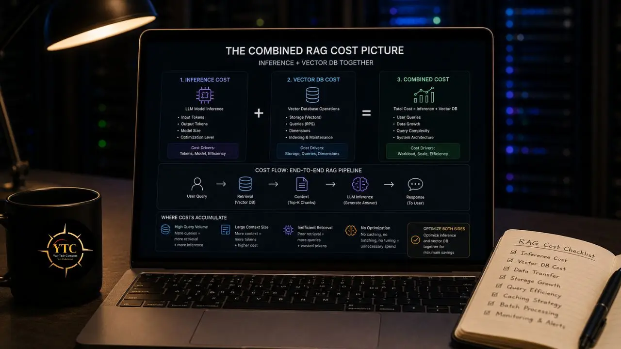
Understanding inference optimization and vector database costs separately is useful. Understanding how they interact is essential.

Here’s the interaction that most teams miss: a poorly configured vector database with a high recall miss rate can force your LLM to work harder. If your retrieval system regularly misses relevant context chunks, you compensate by using longer prompts; more context is passed to the LLM to increase the chance of covering the missing information.

Longer prompts mean more input tokens. More input tokens mean higher inference costs. Retrieval quality, therefore, has a direct effect on your inference bill.

The recall-cost interaction makes this more concrete: for example, a system at 95% recall misses 1 in 20 relevant documents. At 99% recall, it misses 1 in 100. That difference can determine whether your RAG system regularly misses important context or almost never does. Teams that optimize inference while ignoring retrieval quality often end up spending more on inference because the LLM is being asked to compensate for context gaps that better retrieval would have avoided.

The same is true for latency. A RAG pipeline with slower retrieval and slower generation can easily miss user-facing performance targets, even if each piece looks acceptable on its own. The two systems need to be co-designed for latency, not just cost.

The Full RAG Pipeline Cost Breakdown Per 1,000 Queries (Approximate)

The LLM cost dominates across all scale tiers, which means model routing (sending appropriate queries to cheaper models) delivers the highest dollar-per-engineering-hour return of any optimization. Vector DB cost is a rounding error when configured efficiently. But the efficiency of the vector retrieval layer determines whether your LLM costs compound or stay controlled.

The Optimization Priority Order: Where to Start

This is the sequence that tends to deliver the fastest payoff for many teams, based on production patterns across AI infrastructure. Apply it in order, measure quality after each change, and stop when the economics work for your workload.

For Startup Teams (<$5K/month AI spend)

First: Enable continuous batching if you are self-hosting, or switch to a managed inference provider that supports it. This is often one of the highest-impact changes for the least engineering effort.

Second: Start with pgvector if you are already on Postgres. Do not add a dedicated vector database until your corpus or latency requirements clearly outgrow what pgvector can deliver. Managing one database is simpler than managing two.

Third: Add observability before you add deeper optimization. You cannot prioritize correctly without knowing where your costs are going. Track token consumption per feature, vector database query latency, and retrieval recall rate separately.

For Growth-Stage Teams ($5K–$50K/month)

First: Apply FP8 quantization if you are on H100/H200 hardware. On modern GPU generations, this can deliver meaningful speed gains with limited impact on quality, depending on the model.

Second: Implement model routing. Separate your query types: simple queries, such as FAQ, classification, and extraction to a cheaper model, and complex queries to a frontier model. Validate quality metrics per route, not just overall.

Third: At larger vector counts, evaluate whether a managed vector database still justifies its premium versus a self-hosted alternative. Run the math for your specific scale: GPU or VPS cost plus operational time versus the managed monthly bill.

Fourth: Implement hybrid search if you have not already. Pure vector search rarely stays sufficient on its own. As RAG systems mature, hybrid retrieval often becomes the practical default, so it is better to plan for it deliberately than to bolt it on later.

For Enterprise Teams ($50K+/month)

First: Evaluate self-hosted inference on H100s. The break-even point against managed APIs depends on utilization, staffing, and reliability requirements, but it can become attractive at higher spend levels.

Second: Implement speculative decoding for your highest-volume text-generation workloads. The throughput gains can be significant when the workload is well-suited to it.

Third: Commission task-specific distillation for your top two or three highest-volume query types. Well-distilled 7B–20B LLMs can cover a large share of single-turn chat and reasoning traffic for many applications, depending on the task. Identify which workload categories fit that pattern and distill for those first.

Fourth: At very large vector counts, evaluate whether self-hosted infrastructure or a managed vector platform makes more sense for your team. The right answer depends on cost, operational maturity, and the level of platform engineering capacity you can sustain.

For teams building enterprise AI workflows that need to understand how agentic AI tools fit into the cost picture alongside inference infrastructure, our Claude Cowork review explains how agentic AI tools create their own inference cost patterns through multi-step workflows. And, for the broader AI policy landscape, particularly for teams operating in or planning for African markets where compute infrastructure and AI governance intersect, our AI policy in Africa guide and our AI in Africa section provide essential context. In addition, our AI Unboxed section tracks the latest model and infrastructure developments as they affect inference cost economics in real time.

FAQs

Conclusion

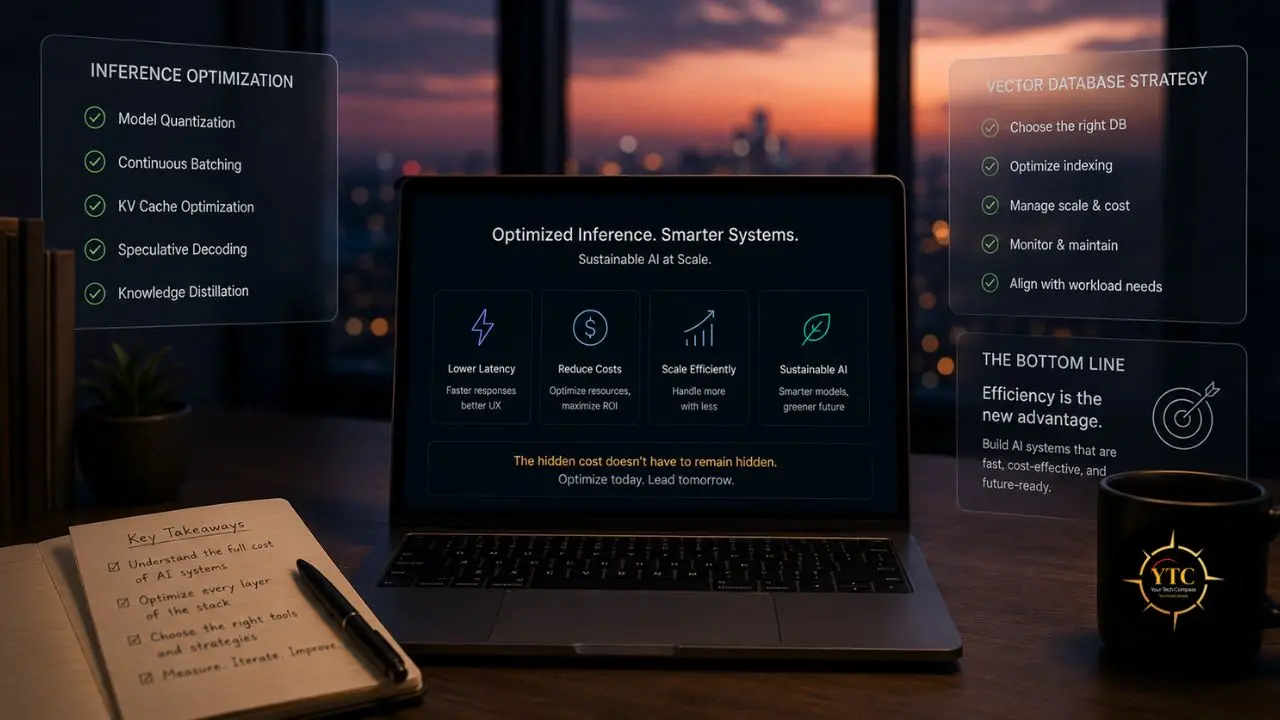
The teams that build sustainable AI products in 2026 aren’t the ones with the best models or the most GPU access. They’re the ones who understand the cost structure beneath the models and manage it deliberately. Inference optimization and vector database architecture are not infrastructure details to defer until you’re at scale. They’re the architectural decisions that determine whether your unit economics are viable when scale arrives, and scale, for any successful product, arrives faster than the cost model was written to handle.

The practical path forward is simpler than the technical depth of this guide might suggest. Start with measurement: token consumption per feature, inference latency per model tier, vector database query latency, and retrieval recall rate. Apply quantization and continuous batching before anything else; they deliver the highest ROI for the lowest effort. Route queries to the cheapest model that handles them adequately. Default to pgvector until scale demands more, and choose your vector database upgrade path based on your team’s infrastructure capacity, not vendor marketing. The 23× cost difference between naive and optimized AI infrastructure isn’t a theoretical number. It’s the gap between a product that compounds in value and a product that compounds in cost.

Every AI infrastructure guide, tool review, and honest technical breakdown worth bookmarking lives at YourTechCompass.com, where we give you the verified numbers and the decision frameworks that the pricing pages won’t.